MicroPhysics

Flexible Magnetic Media Surface Roughness Characterization:

Contact Interferometry with a Hertz Pressure Loader

Christopher Lacey

MicroPhysics, Inc.

Introduction: 
Contact interferometry is a superior technique to evaluate the surface topography of flexible media.  In this technique, the flexible media is loaded against a transparent surface under a known contact pressure.  The spacing between the flexible media and the transparent surface is primarily due to the surface roughness of the flexible media. Under higher contact pressures, the tape surface becomes smoother and the spacing decreases.   The relationship between contact pressure and average spacing has been called “tape surface compliance.” Other surface measurement methods such as non-contact interferometry, stylus profilometry, and AFM are not able to fully characterize how the media surface behaves as a function of contact pressure.

The purpose of this technical note is to describe a method for the determination of tape surface compliance. The method is broken into three parts: (1) the application of known contact pressure to the media, (2) the measurement of spacing with the contact pressure applied, and (3) the reduction of spacing information to parameters which indicate the variation of tape surface roughness as a function of contact pressure.

Throughout this work, “spacing” refers to a value which is spatially averaged.  Although true contact occurs at the peaks of the media surface roughness, the (averaged) spacing is typically non-zero. 

To determine the compliance relationship, a pressure cell was constructed using a polyurethane hemisphere to load flexible magnetic media against a flat glass window.  The contact pressure between the hemisphere and the glass window was calculated using the theory by Hertz.  MicroPhysics Tape Spacing Analyzer was used to measure average spacing between the tape and the glass window under a range of contact pressures.  A functional relationship between average contact pressure and average spacing was established by fitting two coefficients using a least squares technique.

Pressure Cell:
The pressure cell is shown in Figure 1.

Figure 1: Pressure cell For use with contact interferometer

Flexible media was placed between the glass plate and the urethane hemisphere.  The contact pressure was applied by loading the hemisphere against the fixed glass plate using the motorized Z-stage.  As the Z-stage was raised, the force pressing the sphere against the plate increased and the area of contact between the sphere and the plate also increased.  The load force was measured using the load cell and the area of contact was measured by observation through the glass plate using the MicroPhysics Tape Spacing Analyzer as a measuring microscope.  Table 1 gives the area of contact as a function of load force for the system.

Table 1: Characteristics of pressure cell

Table 1 also gives the average and maximum pressure calculated using the theory by Hertz [1,2]. According to the theory by Hertz, the pressure profile is a hemisphere with the maximum pressure equal to 1.5 times the average pressure. 

The maximum contact pressure ranges from 0.48 to 1.61 atm.  This range is considerably higher than the range obtained by stretching media over a cylindrical contour [3].  The maximum pressure obtained using that method was on the order of 0.5 atm.  Since the contact pressure at the head/tape interface can be in excess of 1 atm, the measurements made using this pressure cell are closer to the range of interest than those made by stretching the media over a cylindrical contour [4].

For all measurements in this technical note, the measurement spot was placed in the center of the contact patch where the pressure is maximum, and the pressure over the entire measurement area was assumed to be the maximum pressure.  The validity of this assumption was investigated by calculating the pressure distribution in the area of measurement.  The measurement area was square with the sides 0.265 mm long.  Figures 2 and 3 show the calculated pressure distribution in the measurement area for the low and high pressure cases.

Figure 2: Calculated pressure distribution for low pressure case

Since the measurement area is small compared to the contact area, the change in contact pressure over the measurement area is small.  Table 2 gives statistics of the pressure distribution in the measurement area for these two cases.

  Figure 3: Calculated pressure distribution for high pressure case

Table 2: Statistics of pressure distribution

As indicated in Table 2, the contact pressure has little variation over the measurement area.  Therefore, the maximum pressure was used for all calculations.

Spacing Measurement:
To measure spacing between the flexible media and the glass plate, the optical techniques of interferometry and ellipsometry were utilized.  The interferometer optically measures spacing.  In order to measure spacing, optical properties of the flexible media are required.  These properties are measured using ellipsometry.  For the data in this paper, MicroPhysics Tape Spacing Analyzer was for the interferometric measurements and the ellipsometric measurements were performed by the Rudolf corporation.

Interferometry:
Microphysics Tape Spacing Analyzer (TSA) is typically used to measure head/tape spacing by replacing either the head or the tape with a transparent replica.  A diagram of the system is given in Figure 4.

Figure 4:  Two-Color Interferometer Apparatus

Light leaves the strobe and is directed to the head/tape interface using a beam splitter.  Multiple reflections occur at and between the head and tape surface.  The light then goes back through the first beam splitter to a second beam splitter that directs light toward two digital CCD cameras.  Interference filters of a 10 nm bandwidth are used to produce two distinct wavelengths: one color for each camera.  The system controller processes the intensity information from each camera and feeds the data to the host computer for analysis using multi-beam interferometric theory with corrections for phase shift on reflection.  Head/tape spacing can also be measured using real heads in conjunction with transparent tape.  When using real heads, the heads are mounted below the tape rather than above it as shown in Figure 4.  

Interferometric Theory: 
Head/Tape spacing is calculated using multi-beam interferometric theory (Equation 1)[5].

                                                     ( 1 )

In Equation 1, r is the amplitude of the external reflection off the lower surface, s is the amplitude of the internal reflection off the upper surface, and is the phase shift between the two reflected wave fronts.

                                                              ( 2 )

In Equation (2), h is the head/tape spacing, is the wavelength of the light, and is the phase shift on external reflection.  The values of r, s, and are typically determined by ellipsometric measurement of the surfaces.

Typical intensity vs. spacing curves for a system with 546 and 633 nm wavelengths are shown in Figure 5.

Figure 5: Typical intensity vs. spacing curves.

One of the most important aspects for the interferometric measurement of spacing is the calibration of intensity of the detectors.  The purpose of intensity calibration is to find scale and offset factors that can be used to transform the output from the digital camera into the normalized intensity units of Equation 1.  To calibrate intensity, a number of interferometric images are captured while slowly varying the spacing.  The spacing must vary so that an interferometric minimum and maximum pass by each pixel of the measuring cameras while they acquire images.  The images are analyzed to determine the maximum and minimum interferometric intensities that were recorded during the calibration process.  The measured maximum and minimum are compared to the theoretical maximum and minimum of equation 1 and offset and scale factors are calculated for each pixel on each of the detectors.  These offset and scale factors are used to transform the camera output into the appropriate units for application of equation 1.

When the spacing is determined by application of Equations 1 and 2, the spacing can be determined independently by each color.  Due to system imperfections, the spacing measurements determined by each color can be different.  If the difference between the two measurements is greater than a pre-specified tolerance, the spacing measurement is rejected, otherwise, a degree of confidence is assigned to the measurement.

Ellipsometry:

The phase shift on reflection and the reflectance of the flexible media were determined by ellipsometry.  Four samples of magnetic tape were measured.  The results are shown in Table 3.

Table 3:  Optical Data for Various Magnetic Tapes

In Table 3, ps is f and ref is r.  The values for n and k were obtained from the ellipsometer assuming the flexible media to be an isotropic bulk medium.  The values for f  and r were calculated from n and k using equations given in reference [5].  

The in-line test cases had the machine direction of the magnetic tape in the plane of the light used for ellipsometry.  The transverse cases had the tape rotated 90 degrees (Figure 5).  The differences in the measurements for the two cases are indicative of imperfections in the assumptions used to reduce the data, in particular, that the media is homogenous and isotropic.  For determination of spacing, the average values were used as shown in the last two columns of Table 3.

Figure 5: Transverse and in-line tape orientation in ellipsometer

Spacing Measurement in Pressure Cell:
To perform the spacing measurements for flexible media surface characterization, MicroPhysics Tape Spacing Analyzer (Figure 4) was used with the Hertz pressure cell (Figure 1) substituting for the tape looper.

Measurements:
Measurements of average spacing in the pressure cell were made for four samples of each of the four different tapes.  The spacing measurements were made using a 111 by 111 pixel area of each measurement camera.  This area corresponds to a square with 0.265 mm long sides on the surface of the tape.  The average spacing data is reported in Table 4.

Table 4: Average Spacing Measurements

Each average spacing measurement consists of the average of 12,321 pixels of data in the area of interest.  The standard deviation of the spacing data for each measurement was also recorded.  The standard deviation data is reported in Table 5.

Table 5: Standard deviation of spacing measurement data

In all cases, the average spacing and the standard deviation of spacing decrease as the pressure increases.

Fitting parameters to the data:

The average spacing data was fit to Equation 3

                                                           (3)

where h is the average spacing,  is the contact pressure normalized to sea-level atmospheric pressure, and  and  are fit parameters.  Since  generally has a value between zero and negative one, this equation has hyperbolic characteristics, i.e. it approaches but does not intercept either axis. 

For the purpose of communication and reporting the fit parameters, two other parameters are used:  and .  The parameter  is the spacing at 0.1 atm of contact pressure.  Parameter  is the spacing at 1.0 atm of contact pressure.  Transformations between ,  and  ,  are giving in the following equations.

                                                           (4)

                                                                 (5)

                                                    (6)

The parameters  and  are both expressed in units of length; they can be easily transformed to different systems of units and their interpretation is straight forward.

Values of  and  for the four tapes are given in Table 6.

Table 6: Surface compliance parameters for various magnetic tapes

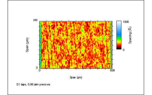
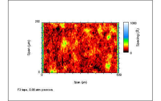
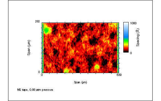
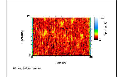
The standard deviations for the measurements were generally below one nanometer, indicating not only that the measurement technique was very repeatable, but also that the surface roughness of the tapes was very uniform.  One exception to the uniformity was the M2 tape which appeared to have small particles on the surface causing increased non-uniformity between different measurement samples.

Data Images:
Contour plots of spacing are given in Figures 6-9.

Figure 6: Spacing for D1 tape at 0.88 atm.

Figure 7: Spacing for F3 tape at 0.88 atm.

Figure 8: Spacing for M2 tape at 0.88 atm.

Figure 9: Spacing for M3 tape at 0.88 atm.

Summary:
This document describes a method and apparatus for the characterization of surface roughness of flexible media.

References:

[1] Burr, Author H., Mechanical Analysis and Design, Elsevier, New York, 1983.

[2] Smith, David P., “Contact and Pressure Relationships of Polyurethane Hemispheres on Glass,” Unpublished Technical Note of 3M Data Storage Tape Technology Division, St. Paul, 1995.

[3] Lacey, C.A., and Talke, F.E., “Measurement and Simulation of Partial Contact at the Head/Tape Interface,” Transactions of the ASME, Journal of Tribology, Vol. 114, October, 1992

[4] Wang, Erik L., Wu, Yiqian, and Talke, Frank E., “Tape Asperity Compliance Measurement using a Pneumatic Method,” IEEE Trans. Mag., Vol. 32, No. 5, Sept. 1996.

[6] Anders, Thin Films in Optics, The Focal Press, London, 1965.

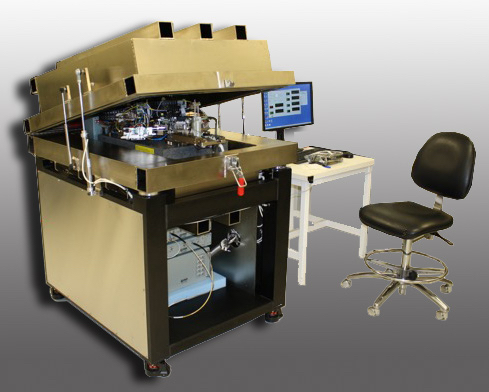
Guzik Spinstand Helium/Altitude Chamber

Flying Height 
Tester

Altitude Simulation Chamber

Dynamic Protrusion Tester

Tape Head Tester

Tape Spacing Analyzer

SliderLab

TapeLabH

TapeLab